About
This section covers some of the more basic functions of the Metrix Asset Management System including:
This section covers some of the more basic functions of the Metrix Asset Management System including:
This page covers some of the basic navigation options available within the core ‘Assets’ page in the Metrix Asset Management system including:
The built-in map window inside the main ‘Assets’ page supports various computer mouse gestures to interact with the map location and view. These are detailed below:
These notes assume a standard right-hand mouse configuration with scroll wheel.
Panning a map means to shift the map image relative to the display window without changing the viewing scale.
To pan the map window, hold down the ’left’ (main) mouse button and drag your cursor. The map will follow until you release the mouse button.
‘Zooming in’ refers to the action of adjusting the view of the map to make a specific area appear larger and closer.
To zoom in, scroll the mouse wheel up.
‘Zooming out’ refers to the action of adjusting the view to make the image or area ot he map appear smaller and farther away.
To zoom out, scroll the mouse wheel down.
‘Map rotation’ is a way of viewing the map window from a different orientation.
To rotate the map view, hold down the ‘right’ mouse button and drag your cursor to the left of the map window. The map will continue to rotate in a clockwise direction until you release the mouse button.
Note: to rotate counter-clockwise, drag the cursor to the right.
‘Map tilt’ refers to the angle at which the map is being viewed from. By default, the tilt is ‘flat’ and being viewed from directly above. When ’tilted’, the map view is angled so that the user feels they are looking ‘along’ the map.
To tilt the map view, hold down the ‘right’ mouse button and drag your cursor up to the top of the map window. The map will continue to tilt until you release the mouse button.
Note: to reverse the tilt, drag the cursor down.
In order to interrogate an asset via the main ‘Assets’ page map window, pan & zoom the map window to the asset location and single click (left-click) on the asset’s spatial feature.
Remember, click and drag will pan the map. Single click to use the Info Tool.
The info panel will appear/populate on the right hand side of the map window when one or more valid features have been interrogated by a click.
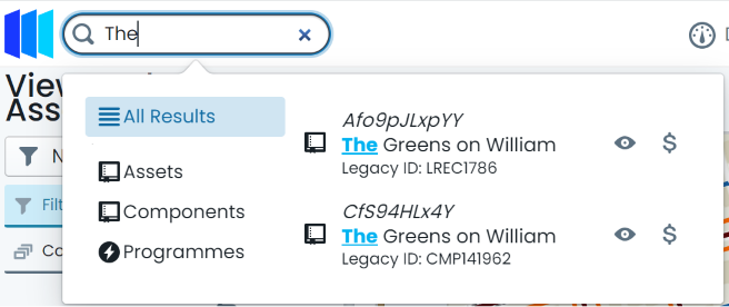
In addition to basic pan and click operations, the Metrix Asset Management system contains a free text search tool that can navigate and select chosen results for you. To start a search, simply click inside the search pill at the top of the page, and begin typing your criteria. The following asset/component fields are included in the search index:

The search tool will begin looking for results immediately and render them in a box below the search pill. By default, ‘All Results’ will be shown. Users can however, refine their results to the following result levels:
This section details the info panels available within the core ‘Assets’ page in the Metrix Asset Management system including:
In addition to the above panel structures, various tools built into these information panels are also detailed, including:
The component info panel displays information as it pertains to the selected/active component. The component info panel has the tab title of ‘Info’. The following sections are included in the component info panel.
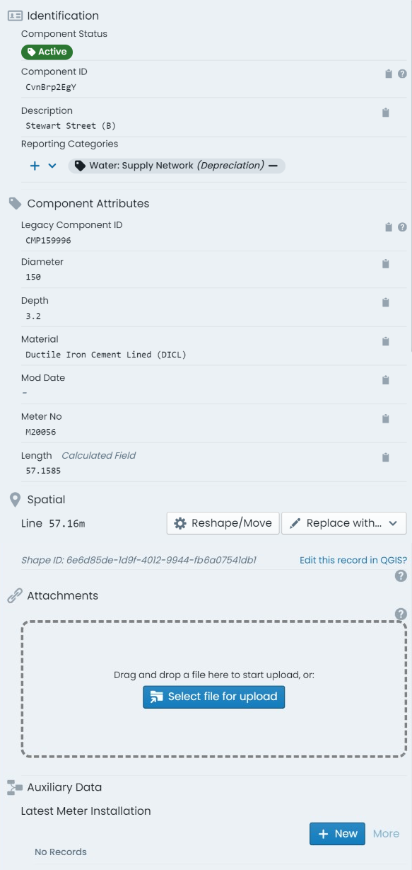
Contains identifying information for the component including:
Renders the custom form definition assigned to the component’s component group (if any). Each form field will be displayed in accordance with the form definition’s layout specification.
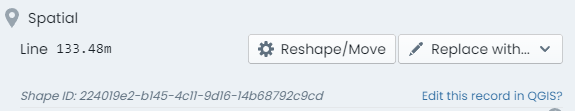
Provides basic information about the component’s underlying spatial feature as well as access to tools to update or replace the geometry definition. Additionally, the unique Shape ID value for the spatial record is displayed at the bottom of this section.
Displays a panel where users can interact with existing component attachments and upload new attachments. Any existing attachments can be clicked on to view, download, or manage. Users can also simply drag and drop files into this section to create new attachments against the component.
Renders a list of task records attributed to the component. Users can also create new task entry from this section.
The intervention info panel displays information as it pertains to the lifecycle metrics of the selected/active component. The intervention info panel has the tab title of ‘Intervention’. The following sections are included in the intervention info panel.
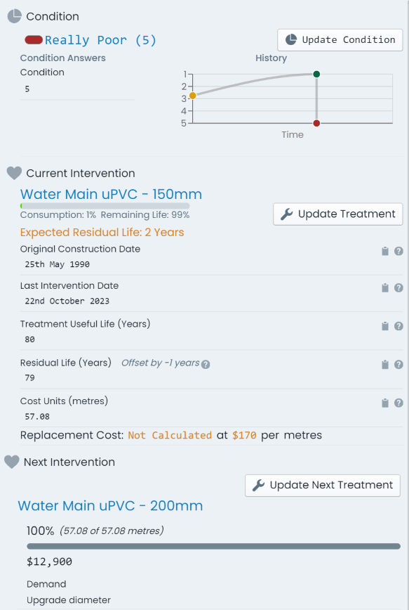
contains information about the latest condition assessment for the component. Additionally, a button (‘Update Condition’) is provided for updating the condition with a new assessment. Lastly, a graph displaying the change in condition over time is presented for context.
contains information about the current state of the component including:
Additionally, this section contains a button (‘Update Treatment’) linking to a panel that allows users to update the current intervention treatment.
contains information about any slated next intervention treatment definition. The recorded intent and scope of the next intervention is detailed alongside a button (‘Update Next Treatment’) linking to a panel that allows users to update the next intervention treatment.
The transactions info panel displays information as it pertains to the financial transaction ledger of the selected/active component. The transaction info panel has the tab title of ‘Transactions’. The following sections are included in the transactions info panel.
contains a snapshot of the current ‘Gross Value’, ‘Depreciable Value’, ‘Accumulated Depreciation Value’, and the ‘Carrying Value’. These figures represent the financial position of the selected/active component including all of its active financial transaction ledger postings.
When an intervention treatment has been assigned to the component, and valid rates exist, the ’ value summary pills also display a calculated value field based on the relevant rates and residual life.
provides an interface for users to view and manage the selected/active components depreciation settings - which are optional and, presently, for information purposes only. Users can view/set the depreciable value of the component as either a fixed value, or a percentage share of the components gross value. Likewise, users can set the annual depreciation rate for the component as either a fixed value, or a percentage share of the components value.
this sections provides a table view of every active financial ledger transaction posted against the selected/active component. Each row details the transaction type, finance category, posting date, and posting value of the entry. Additionally, each row has an option to delete the transaction posting (if permitted).
The option to delete a transaction posting is only permissible in the following circumstances:
Lastly, above the transaction history table, reside options to create new financial ledger transaction entries (‘New Transaction’) as well as performing a financial reclassification (‘Reclassify’) of the component.
![]()
![]()
The programming panel displays details on any mobile programmes that the selected/active component is an item within. For each related programme, users are provided with an overview of the programme name, due date, and current completion status.
Clicking on a programme item will bring up a panel providing additional information about the component item within the programme.
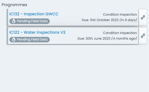
Elements of the Programme system are still flagged as beta products. As such, some of the items and information accessible through this panel are subject to change.
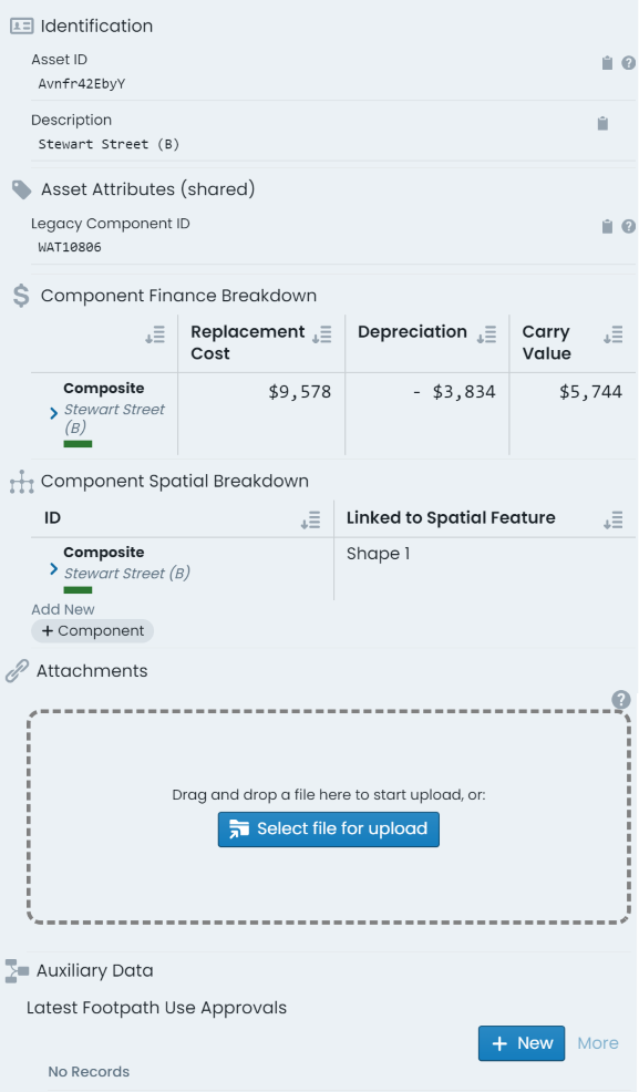
The parent asset info tab provides information pertaining to the parent asset of the selected/active component. The parent asset info panel has the tab title of ‘Parent Asset’. The sections detailed below are included in the parent asset info panel.
Consider a road asset with three (3) components - earthworks, base, and surface. Each of the components would have their own unique component info panel, intervention info panel, transactions info panel, and programming info panel. That is, each time you change the active component, the information contained within these panels will update to reflect the new entity.
The parent asset info panel is constant regardless of the active component. The information displayed on this panel will only change when a different asset is activated. Likewise, any details edited on the parent asset info panel will persist for any of the ‘sibling’ components across the asset. That is, the information is shared.
contains identifying information for the asset including:
renders the custom form definition assigned to the asset’s classification (if any). Each form field will be displayed in accordance with the form definition’s layout specification.
The ‘shared’ reference in the section’s header is simply communicating that the information within this panel is shared across all child components of the asset.
as each component within an asset can be defined by either a common/shared geometry, or a distinct geometry to that component, the component spatial breakdown provides a context for the spatial features used across the asset..
displays a panel where users can interact with existing asset attachments and upload new attachments. Users can interact with existing asset attachments and upload new attachments. Any existing attachments can be clicked on to view, download, or manage. Users can also simply drag and drop files into this section to create new attachments against the asset.
renders a list of task records attributed to the asset. Users can also create new task record entries from this section.
This section discusses the following info panel tools that exist and/or can be used regardless of the specific info panel you are viewing at the time. These tools are situated above the core info panel sections and are always visible (whilst the info panel is open).
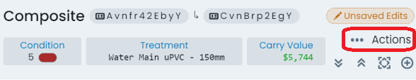
The ‘Actions’ menu contains a list of asset and component related actions that can be completed using
the system. Depending on the selected asset and/or the active component, various options in the actions menu
will be enabled and disabled.
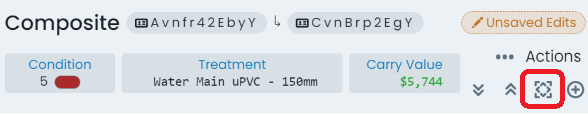
The ‘Zoom to Component’ button is located in the top-right hand corner
of the info panel, outside of any other content panels (i.e. component info panel, transaction
info panel, etc.). When clicked, the map window will pan and zoom to reveal the extents of the
active component.
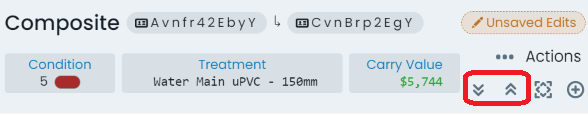
The expand and collapse options provide users with the ability
to collapse all of the info panel sections into flatter, header only, sections. This can be useful on smaller
resolution monitors, when looking for a certain section header. Conversely, the expand button will
display every info panel’s content.
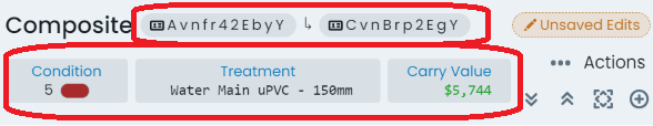
The shortcut pills give quick and easy access to core data like condition,
carrying value, and ID values. Furthermore, clicking on the pill will take users through to the
appropriate info panel for further information.
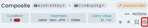
The ‘Add to Collection’ tool allows users to include the selected/active
component in the current (or new, if none is current) collection set. Note: When the component is already
included in the collection set, this button will change to ‘Remove from Collection’.
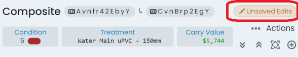
When the selected/active component has been modified, this pill acts as a menu that
renders information about the data that has been modified (when clicked). Further to this, users can
revert any pending changes against the selected/active component by clicking ‘Rollback’ in this menu.
At the very top of the info panel, next to the classification label, exists a settings button that will take users through to the classification configuration page for the selected/active components classification.

To close the info panel completely, simply click the ‘X’ icon in the top-right hand corner of the info panel.

On the left-hand side of the info panel is the active component switcher. This side panel displays all of the assets components, with the current active component highlighted. Users can simply click on a different component in this list to switch the info panel to displaying information about that component. Furthermore, this panel also lists component groups that exist on the asset classification definition, but do not have any assigned components.

Throughout all of the info panels, on the right-hand side of any data field, users will find the ‘Copy Field Value’ button. This will put the value contained in the adjacent field into the users clipboard.

The Metrix Asset Management system provides built-in access to publicly accessible aerial photography imagery as well as basemaps as backdrops to your asset portfolio. These layers provide users with helpful context on the area they are viewing in the map window. To further assist with seeing asset content in association with these layers, Metrix also contains some tools to modify which backdrop you are seeing, as well as the colour intensity of the backdrop in comparison to your asset portfolio.
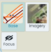
For nearly all users, there exists a colour combination that is hard to decipher between and thus difficult to read when displayed in a map window. To cater for this, the Metrix Asset Management map tools provide users with the ability to put the map backdrop into ‘Focus Mode’. This will binarise (to make black-and-white) the backdrop so that the colours of your asset portfolio are easier to distinguish.
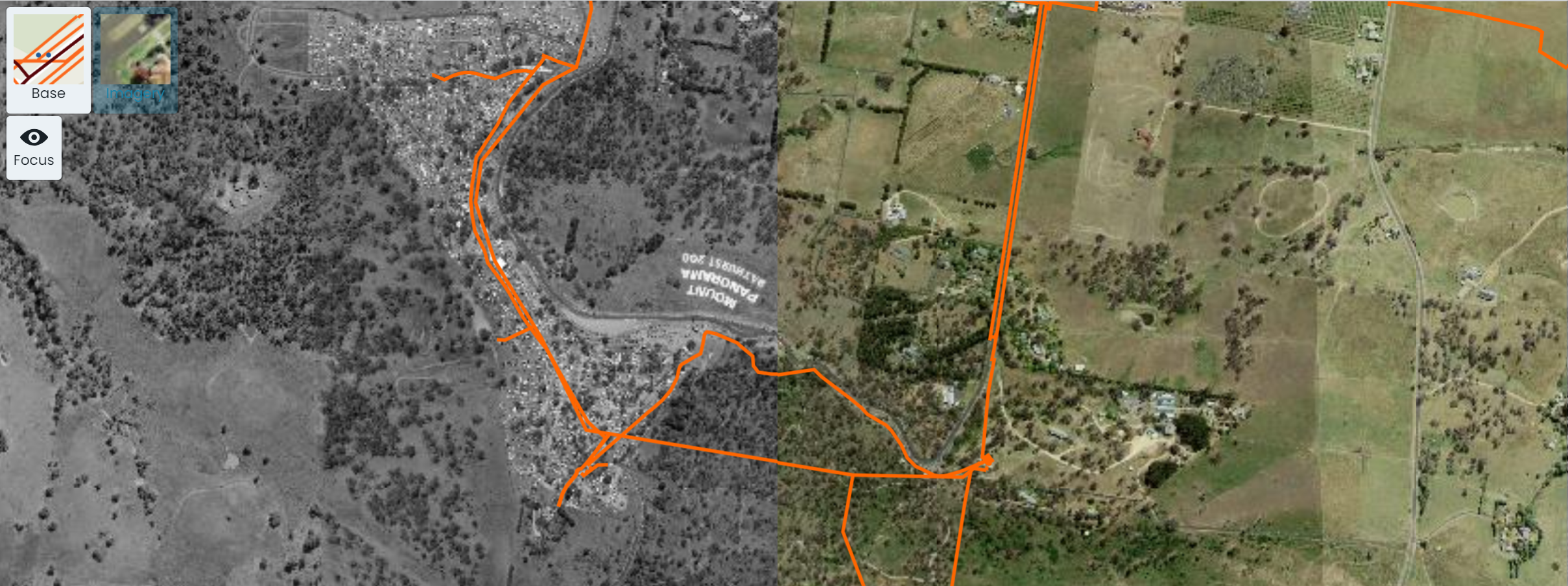
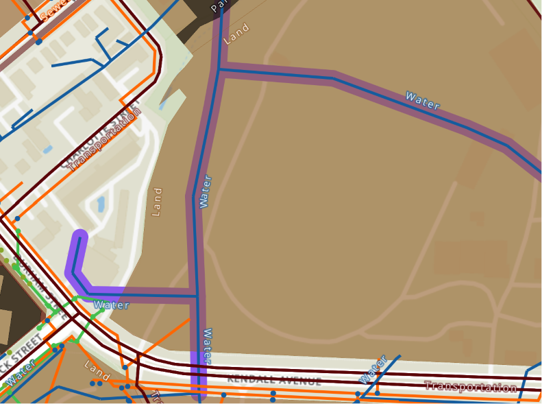
To view the aerial imagery as a backdrop to your asset portfolio, simply click on the ‘Imagery’ button in the top-left hand corner of the map window. This will swap out the underlying view to the aerial photograph imagery configured for your environment. The screenshot below shows a map window with aerial imagery as the backdrop, split between focus mode and standard.
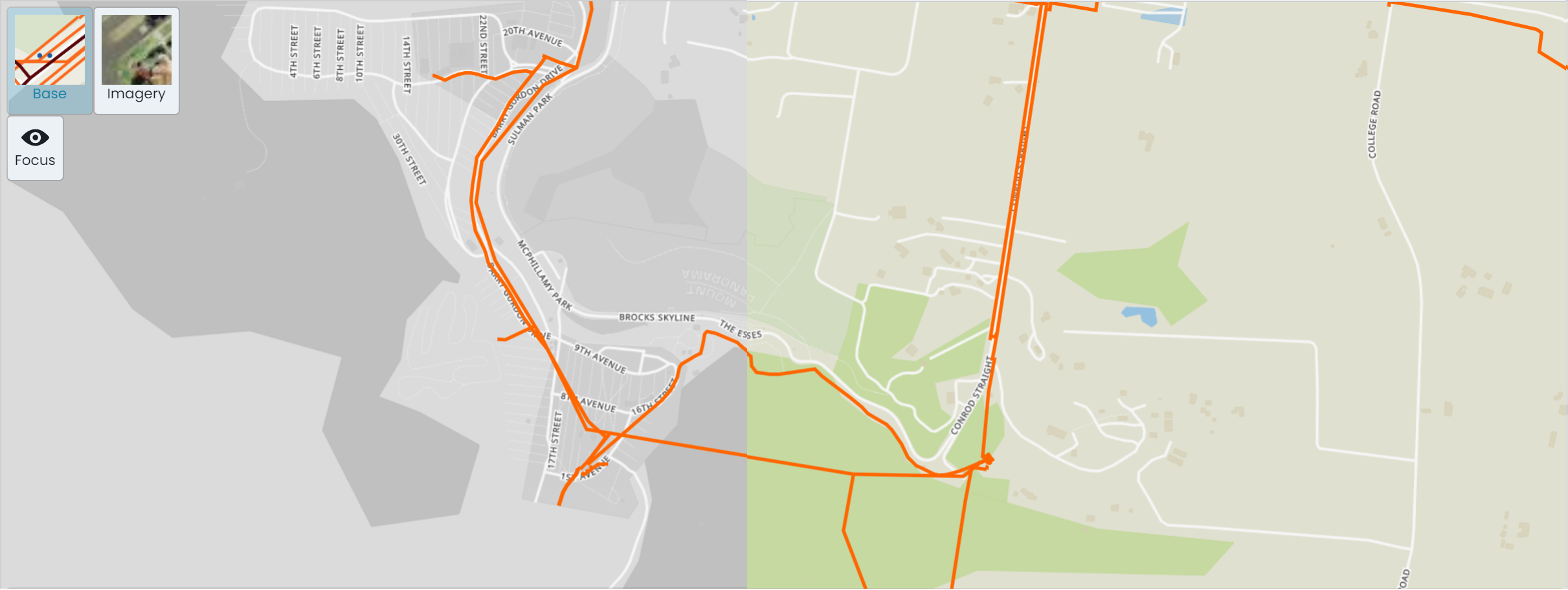
To view the basemap as a backdrop to your asset portfolio, simply click on the ‘Base’ button in the top-left hand corner of the map window. This will swap out the underlying view to the basemap configured for your environment. The screenshot below shows a map window with basemap as the backdrop, split between focus mode and standard.
The Metrix Asset Management system is equipped with a built-in data filtering tool that works across a variety of pages and functions within the system. This allows users to create and manage subsets of their entire asset portfolio for viewing, reporting, as well as sharing with other users of the system. Additionally, the data filtering tools can aid in highlighting asset management targets within your asset portfolio - filters can be combined to create multiple restrictions on included components.
Filters can be used to find ‘problem’ assets, or those that may require review for capital intervention. For example, you could build the following filter to find expiring road surfaces:
Applying the above filter will restrict the displayed components to only those meeting this criteria.
Once a filter has been configured, users can choose to save that filter for later reuse. Saved filters can also be shared so that all users of the system can leverage that filter set.
Saved filters will regenerate matching results every time they are selected. That is, the parameters are saved for reuse, not the list of result components. This means users can save a filter, and check back in on the components that fall in and out of its result set over time!
In addition to the core ‘Assets’ page map window, the filter tool works across the Metrix Asset Management system in areas such as:
This means that users can define a filter once, and then, view dashboard widgets as they pertain to that reduced data set only. Further more, users can create a filter and then export the results of that filter to a CSV report by choosing the filter in the reports page.
The following options are filterable in the Metrix Asset Management System:
The Metrix Asset Management system is equipped with a built-in map theming tool that works automatically with your data and attributes. This allows users to visualise breakdowns of their entire asset portfolio, assisting in better and faster decision making. Additionally, these visualisation tools can aid in highlighting asset management targets within your asset portfolio.
Remember, the Metrix Asset Management system controls spatial features at a component level. When viewing some map themes, there may be overlapping shapes caused by stacked geometries of multiple asset components. This can cause obscuration and/or blending of the rendered colours.
In these cases, it is advisable to filter your data to a specific component group.
There are a number of built-in map theme visualisations that are ready to work immediately for you. These cover a range of areas from lifecycle theming, to report category visualisations. The following details some of the available themes. This is not an exhaustive list, but provided for context on the types of themes provided.
These map themes switch around the asset classification and status.
This is the default visualisation theme for the system. Each component is coloured according to its Asset Class (the first level of the asset classification structure).
This theme colours according to the Component Group level of the classification structure. This offers far more granularity than the Asset Class theme.
Users should be aware of potential stacked geometry issues when using this theme.
The status theme colours each component geometry according to its current status code.
These map themes aim to highlight the lifecycle metrics associated with your asset portfolio.
The condition theme displays components on a colour gradient from green (1 - excellent) to red (5 - really poor).
This theme converts a component’s residual life to a percentage of its overall useful life. The result is then displayed on a colour gradient from green (100% remaining life) to red (0% remaining life).
This displays components in a accordance with their recorded original construction date. This is a useful data audit tool as it will highlight anomaly records (in comparison to the surrounding asset components).
The system takes each of your configured report category configurations and automatically creates a map theme to render each component in accordance with their assigned option within that category (including missing or no assignments).
The map theme switcher will render an option for each configured report category.
The custom attribute form specifications contain several restricted attribute names that relate to component metrics such as width, length, height, etc. If any of these fields are implemented within your component custom attribute definitions, the map theme generator can style your geometries based on these numeric results.
Any custom attribute definition that is controlled by an option list will be available within the map theme switcher for render.
The concept behind collections within the Metrix Asset Management system is to allow users to choose various components from a map or list, and build an actionable group from them. A collection, in other words, is a selection set that users can use in system actions.
Once a collection set has been constructed, users can use that collection to:
When a component is included in a collection set, the spatial feature will be rendered with a halo, highlighting it to the user.
As mentioned in the above list, collections can be converted into permanent custom filters. User can also start a collection from the components resulting from an existing custom filter. There is a two-way interoperability at play here.
An elemental facet of the Metrix Asset Management system is spatial representation of asset components. At a basal level, this is enforced by the mandatory requirement that every component maintained in the system MUST reference a valid spatial feature. The system has been built around the existence of spatial features, and several tools exist to make this both beneficial, and easy for end users, including:
Each spatial feature in the system is its own record. That is, the geometry is not ‘just’ another attribute of the asset component. Instead, by maintaining spatial features as distinct entities, we are able to ’link’ a single geometry to more than one component. This means, you can have the same line feature representing the earthworks, base, and surface of your road asset. Editing the line once, will update the representation for all.
It should be noted, however, that this sharing feature is not mandatory. Within an asset, each component could have their own distinct spatial representation. YOu could even maintain a hybrid approach, with two components sharing a geometry, whilst a third maintains a distinct feature.
The only caveat is that geometries cannot be shared across components with different asset parents. The relationship must stay within a single asset.
The system come with built-in spatial editing tools for basic geometry creation and updates. These tools are simple to use and support all simple geometry types; points, lines, and polygons. In the case that your geometric construction requirements are more advanced that those offered in system, the Metrix Asset Management system has published a free to access QGIS plugin that can connect to your cloud environment (using your Metrix account details), view your geometry data, as well as make edits and save changes back to the system.
A workflow that many users implement is to initialise an asset its components in system first, and then switch to using the QGIS plugin to refine and align the new features accordingly.
With such a strong relationship to underlying spatial features, the Metrix Asset Management system is able to leverage geometric principles in offering advanced asset management operations, in an easy to use and understand package. Such an operation is the ability for users to SPLIT assets or components at a given point with the system handling all the financial apportionment of capital value for them. This is great for recording partial renewals, re-segmenting your network assets to cater for additional installations.
Another added benefit of mandating spatial features is the ability to leverage spatial properties as attribute information. See smart attributes for more information.
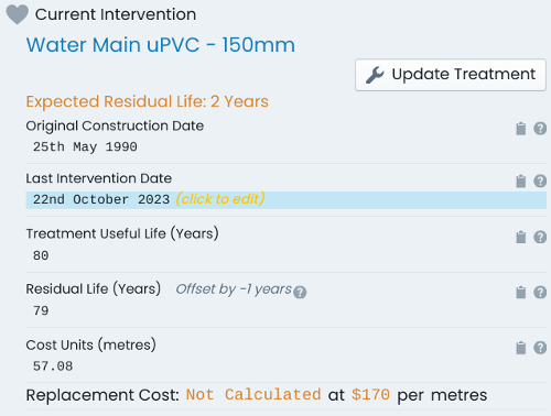
In simple terms, the Residual Life is the number of years that a Component has left/remaining before a capital intervention is required. The Residual Life is calculated as the difference between its useful life and the Component’s age plus any residual life offsets (see below) recorded against the Component.
As a Component goes through it’s life, it is expected that it will degrade/age over the years. How any particular Component experiences this ageing process however, will be in accordance with some very local factors relevant to that Component only. This means that any one Component could under-shoot or exceed it’s expected useful life - it also exemplifies how a Component’s useful life is just an averaged expectation, rather than a hard-and-fast rule.
To cater for such variations to lifecycle patterns, the system allows for the Residual Life to be ‘set’ by the user at any point throughout the Component’s life cycle. That is, the user does not modify the useful life of each Component, but rather, can set the residual life to the value they see fit.
This translates to a residual life offset being inferred upon the Component. This residual life offset takes effect upon the calculated residual life by being added to the calculated residual life.
It is for the reasons stated above, that the formula for Residual Life in the Metrix Asset Management system is:
$$ [UsefulLife] - [Age] + [ResidualLifeOffset] $$It is important to remember however, a Component will NOT start ageing until it reaches it’s Initial Capital Anniversary date. By default, this is 30 June and is listed in the ‘Intervention Statistics’ section of the Component info panel.
Further to this, it is important to note that adjustments to a Component’s Residual Life only begin taking effect once the Initial Capital Anniversary date has passed. This is simply because, as mentioned above, the Component does not commence ‘ageing’ until it passes this date.
The following provides additional details on the inputs to the residual life formula discussed above.
A component’s residual life offset is an offset applied to the calculated ‘residual life’, to either increase or decrease the resulting value. The residual life offset is calculated by the Metrix Asset Management system as the difference between the calculated ‘residual life’ and the subjectively assessed remaining life. That is:
$$ [Assessed Remaining Life] - [Calculated Remaining Life] $$Consider the road surface component of a road Asset that has a useful life of 15 years. Now consider that the age of the Component is 10 years. This means that the residual life (using the formula above) is:
$$[Useful Life] - [Age] + [Residual Life Offset] = [Residual Life]$$ $$15 - 10 + 0 = 5$$Note: at this point in time, the component has NO residual life offset, thus we add zero.
Now assume that at this time, when the component is 10 years old, it is assessed and deemed to actually have 6 years of life left. The system calculates the residual life offset (using the formula above) to be:
$$ [Assessed Remaining Life] - [Calculated Remaining Life] = [Residual Life Offset] $$ $$ 6 - 5 = 1 $$This means that, from now on, anytime the residual life is calculated the calculated residual life will be:
$$ [Useful Life] - [Age] + [Residual Life Offset] = [Residual Life] $$ $$ 15 - 10 + 1 = 6 $$There is NO requirement of a user to consider the concept of residual life offset when altering the residual life of a component. In fact, a user can be safely ignorant of the concepts of residual life offset. All the user needs to supply (going by the above example) is that the residual life of the component should be 6, not 5. The system will take that value and calculate the +1 years offset in the backend.
If the user were to state that the residual life was actually 8, then the system would calculate an offset of +3 years.
As the residual life offset is applied to the residual life value after the initial basic residual life calculation takes place, the reported residual life will continue to decrease as time passes. The user does not need to do anything for this, the system will handle it all.
A Capital Anniversary date is a pre-ordained time of the fiscal year when a capital asset undergoes an ageing event. By default, Metrix environments are configured for annual (once per year) capitalisation. - however, this can be adjusted to suit the needs of the organisation to frequencies such as quarterly, monthly, or the like.
When a Component is first built, or renewed, it will receive a construction date and/or a last intervention date. The Capital Anniversary event relevant to this date is:
Throughout the Component’s life, two other Capital Anniversary events are continuously relevant to the Component - the Most Recent Capital Anniversary and the Next Capital Anniversary:
All of the above Capital Anniversary dates are listed in the ‘Intervention Summary’ section of the Component info panel.
A component’s age is calculated as the difference between the first ‘capital anniversary’ that occurred after the component’s intervention date, and the most recent ‘capital anniversary’ to have passed.
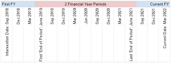
Consider a Component whose last intervention date was 1 September 2018. Also, assume that the current date is 1 March 2022. The component first starts ageing on 30 June 2019 (the first ‘capital anniversary’ following its intervention date), and the last ageing anniversary for the component is 30 June 2021 (the most recent ‘capital anniversary’ to have passed). The Component is therefore 2 years old.
Reports generated from the system support returning the age of a component at a date other than the current date. A report generated at a date of 2 years in the past, will return the age of the component at that date - not today.
The last intervention date refers to the date in which a component last underwent capital intervention works relating to it’s treatment. This includes:
Consider the road surface for a brand new road Asset. After it is first built and commissioned, the Last Intervention Date will be equal to the ‘original_construction_date’. Years later, the road surface will require a reseal treatment. After this reseal (a major renewal intervention), the last intervention date will be the date that this reseal occurred.
The original_construction_date will NOT change following an intervention (i.e. a reseal for a road surface). Only the last intervention date will change over the course of a component’s lifetime.
The quantity/size of a component in the Metrix Asset Management system is stored within the ‘Cost Units’ value, in the ‘Intervention’ info panel. Given that component shapes and measurement techniques differ from type to type, and the method of ascribing a cost to that shape/technique is variable, the cost units value of a component is not restricted to a specific component metric such as length, area, volume, etc. Rather, the cost units number field is free to represent whatever quantity that is required to satisfy the assigned intervention treatment.
The cost method merely controls the calculation configuration for replacement cost. To perform the calculation, the treatment must have an assigned Unit Rate relative to the cost method. Also, the Component must have a valid ‘Cost Units’ multiplier - in the correct Unit of Measure defined by the treatment - for that Unit Rate.
Metrix also supports the implementation of cost unit formulas to automatically calculate these values based off the value of certain metric fields. This is covered in another section pertaining to Smart Attributes and Cost Unit Formulas.
Consider the road surface component of a road Asset. The treatment associated with the component is called ‘14/7mm Initial Seal’ and has the following properties:
From this, we can determine that the component’s cost units are measured in ‘Square Metres’ and, given the ‘Cost Method’ is ‘Unit Rate’, the replacement cost will be calculated by multiplying the ‘Unit Rate’ by the ‘Cost Units’.
Given that the road surface is 1200 sq.m, the cost units for the Component is 1200.
Intervention Treatments in the Metrix Asset Management System provide the ability for users to store and manage unit rates and default useful lives for a variety of component interventions. When assigned to a component group, treatment definitions are able to be used to define the current and/or next intervention method for given components.
The current component treatment informs a component ‘Unit Rate’ (for current cost calculations),
the ‘Default Useful Life’, as well as an indicator to the material and/or methodology used in
it’s original construction. The later of these depends on the naming conventions used in
defining
intervention treatments.
A component’s next treatment definition allows for users to record their ‘best guess’ how a component’s upcoming intervention treatment will be conducted. Such definitions can be based on:
The financial transactions ledger within the Metrix Asset Management system tracks the financial consumption and restoration of asset components over their lifetime. This data is then collated in a number of system reports that satisfy the financial reporting obligations of user organisations. The following outlines a number of terms used throughout the system, and how they tie into the financial frameworks in force.
The replacement cost of a component at the time of valuation (or revaluation). Gross value can increase or decrease over the life of a component through intervention actions such as additions or upgrades to the asset component. Another way that gross value increases or decreases is through indexation – this is essentially increasing the value of a component by a percentage amount, typically in line with CPI.
The accumulated depreciation of a component is the sum of all depreciation transactions logged against it over its life time.
The formula for accumulated depreciation is:
$$ \sum [Depreciation Charges] $$In the Metrix Asset Management system, the accumulated depreciation is posted as a NEGATIVE NUMBER to reflect the fact that it is a ‘consuming’ factor.
Consider a road surface Component for a road Asset. The initial gross value for the component is $123,000.
Each year, the component incurs a depreciation charge of -$8,200. After 5 financial year periods (assuming
no other depreciation events occur) the accumulated deprecation would be:
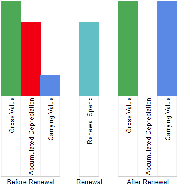
The carrying value of a component is the net worth of the component to the entity in adjusted terms. Carrying value is a calculated value that deducts the accumulated depreciation from the gross value. Given that the depreciation figure is already stored within the Metrix Asset Management system as a negative figure however, the formula for carrying value is:
$$ [Gross Value] + \sum [Depreciation Charges] $$Consider again, the road surface component from the previous example. The accumulated deprecation is calculated
to be -$41,000
The carrying value** for the component after this 5 years period is therefore:
$$ $123,000 + (-$41,000) = $82,000 $$In the Metrix Asset Management system, a renewal expenditure is typically posted as a POSITIVE movement against the components accumulated depreciation. This is to recognise the fact that the action has ‘undone’ the financial consumptions of the past. In turn, the components carrying value (assuming renewal costs equal gross value and a fully depreciated component) is restored to its original gross value as expected.