The Metrix Asset Management system was designed with data interoperability at the forefront. This means
there is a big focus on making it easy to get your asset data in, as well as getting complete and up to date
data out of the system. This section covers the various methods available to export information from the
system, including:
Asset and Component information,
Financial data including movements, and
Useful data extracts
Subsections of Report Generation
About
This section provides background context and requirements of several of the built-in Reports within the
Metrix Asset Management system, including:
Component Data Export: a utility report that is capable of
exporting most of your asset portfolio data.
Financial Movement Report: a report that summarises the
capital value movements of asset components during a specified reporting period.
Indexation Export: a data export that can be used to perform
periodic indexation of component capital value.
Depreciation Export: a data export that can be used to perform
periodic depreciation of component capital value.
Residual Life Report: a data export that can be used to calculate
updated residual life values based on relevant condition assessment results.
It should be noted, that in addition to the above listed reports, the system also contains the following
report options:
Condition Profile: A report that summarises the average condition of components per asset classification.
Latest Condition Report: A report that details the latest condition assessment results for each component in the system.
Programme Report: A report that provides details from a mobile data capture programme.
Calculated Component Value Export: A report that calculates the ‘current’ replacement cost of components based on
the selected intervention treatment, and compares that to the value reported in the financial transactions ledger.
Raw Finance Data: A snapshot of the financial transactions ledger.
Upcoming Component Renewals Export: A report that summarises the ‘Next’ component intervention dates.
Subsections of About
Component Data Export
The ‘Component Data Export’ report is the most comprehensive data extract tool that the Metrix Asset
Management system has to offer. Using the ‘Component Data Export’ will export your information to a single CSV
file, and supports the following features:
Info
This data export can be found under the ‘Data’ section of the Reports Generation page, titled ‘Component Data Export’.
Support for Backdated Report Date
This report type has support for specifying the date in which the report
data should be generated from. Essentially, this allows for users to export
their asset portfolio as it was at a specific time in the past. Where available,
this feature is not compatible with custom filter refinement.
This report type supports the use of a field picker that allows users to expand or limit
the number of report fields included in the export. This can be useful when preparing an
export for an external agency who may not want (or should not see) specific attribute
data.
Custom Attribute Data Inclusion
This report type has support for including custom attribute data from the
asset and/or asset component form definition for included records. Where supported,
this feature will only be available when a custom filter has been selected to
refine the export’s scope of data.
This report type has support for report categories (tags). Where supported,
users will be presented with an option to include or exclude various report
category tags for the data export. If an asset or asset component has been
tagged with the respective report category, it will be populated in an
additional export column.
The ‘Financial Movement Report’ is your principal method of extracting information from the financial transactions ledger within
the Metrix Asset Management system. Using the ‘Financial Movement Report’ will export a summary of your asset component
capital value to a single CSV file, and supports the following features:
Info
This data export can be found under the ‘Finance’ section of the Reports Generation page, titled ‘Financial Movement Report’.
Reporting Period Definition
The ‘Financial Movement Report’ is a special, in that it supports reporting dates as a date range - that is, an ‘opening date’
and a ‘closing date’. This allows organisations to specify the period through which they wish to summarise their portfolio’s
capital value movements via the financial transactions ledger.
The selected dates are INCLUSIVE - start of the day for the ‘opening date’ and the end of the day for the ‘closing date’. A
transaction’s ‘Posting Date’ mandates if it falls inside a selected reporting period.
The ‘Financial Movement Report’, will include the ‘Opening’ & ‘Closing’ capital valuations (gross and accumulated depreciation
value) position for each asset component. For users wanting to understand the financial ‘Movements’ that caused the change in
capital value throughout their opening/closing period, the system includes the sum of all postings made to each configured
transaction type.
Each transaction type (and transaction type effect) will constitute a report column - the value contained representing the sum
of all transactions posted to that specific transaction type throughout the report period.
Users can choose to exclude any transaction types that they know have zero movements throughout the period to simplify the
export, however by default, all transaction types are included.
The ‘Financial Movement Report’ will export a single row per asset component except in the event of a financial re-categorisation
occurring within the report period. In these cases, a row to summarise movements for each affected finance category will be
exported.
If an asset component has undergone a financial re-categorisation during the selected reporting period (opening/closing dates),
then those components will be displayed across two (2) export rows. One row will pertain to the financial movements that occurred
whilst the component was assigned to the original finance category, including the financial ‘write-off’ against that category. Then,
another row will pertain to the financial movements that occurred whilst the component was assigned to the new finance category,
including the financial ‘write-on’ to that category.
This report type has support for report categories (tags). Where supported,
users will be presented with an option to include or exclude various report
category tags for the data export. If an asset or asset component has been
tagged with the respective report category, it will be populated in an
additional export column.
The ‘Indexation Export’ is a helper utility report that generates a valid
Transaction Import Template
with pre-populated indexation transaction types based on supplied metrics. Using the ‘Indexation
Export’ will generate a CSV file that conforms with the import requirements of the
financial ledger transactions import process within the Metrix Asset Management system, including
the following columns:
Component ID,
Posting Date,
Finance Category ID, and
Column headers and transaction values for the indexation-gross and indexation-accumulated depreciation
transactions.
The ‘Indexation Export’ requires the following information. Each is discussed below.
Warning
Merely exporting the report will NOT post the indexation transactions to the financial transactions ledger. Users
must follow the appropriate import steps, with the generated file, to recognise these movements within the system.
‘Indexation At’ Date
This is the date at which you wish to calculate the indexation from. The chosen date value controls:
‘When’ components are considered to be linked to Finance Categories.
‘When’ to calculate each components capital value (gross and accumulated depreciation) at.
Finance Categories
This is the array of finance categories for which you wish to calculate and export indexation movements
for. Any component linked to one of the included finance categories at the supplied ‘Indexation
At’ date value, will be included in the export results.
Indexation Rate
This is the desired rate of indexation (supplied as a percentage) to be applied across the selected Finance Categories. Once
supplied, the system will perform the following calculations:
The above gross and accumulated depreciation values are calculated as at the supplied ‘Indexation
At’ date value. The indexation rate is divided by 100 to convert it to its decimal implication.
Posting Date
This is the date that will be pre-populated into the posting_date column of the exported template.
If the generated report is used to import the indexation transactions, this will be the ‘Posting Date’
for the resulting financial transaction ledger entries.
Cost to Bring to Satisfactory Report
The Cost to Bring to Satisfactory (BTS) report calculates intervention metrics for components based on their
condition a pre-defined factor set. This report works by putting components into groups based on
their assigned report category options (for the chosen report category), and applying a pre-defined
multiplication factor to their aggregated factor bases. A factor base is defined as either the current replacement cost
or the current carrying value of the components - this is defined in the factor set.
Example
For example, taking all of the components assigned to the ‘Roads’ option under the ‘Responsible Manager’
report category, and generating the following results:
Sum of replacement value for components of condition 1, multiplied by a factor of 0%.
Sum of replacement value for components of condition 2, multiplied by a factor of 0%.
Sum of replacement value for components of condition 3, multiplied by a factor of 75%.
Sum of replacement value for components of condition 4, multiplied by a factor of 50%.
Sum of replacement value for components of condition 5, multiplied by a factor of 100%.
Such a report allows asset managers to see a weighted perfective of the condition profile of their asset
portfolio. This report also satisfies part of the requirement for NSW Local Government Organisations to generate the
Special Schedule 7 report.
The report contains the following configuration options:
Support for Backdated Report Date
This report type has support for specifying the date in which the report
data should be generated from. Essentially, this allows for users to export
their asset portfolio as it was at a specific time in the past. Where available,
this feature is not compatible with custom filter refinement.
The BTS Factor Set is a special lookup matrix that is configured for this style of report. By default, the system contains
a standard Factor Set definition that can be modified by users. A valid Factor Set essentially requires:
A report category to be specified, and
For each option within the chosen report category, a percentage based multiplier for a components ‘Replacement
Value’ or ‘Carrying Value’ as specified, for each possible condition score between 1-5.
Depreciation Export
The ‘Depreciation Export’ is a helper utility report that generates a valid
Transaction Import Template
with pre-populated depreciation transaction types based on supplied metrics. Using the ‘Depreciation
Export’ will generate a CSV file that conforms with the import requirements of the
financial ledger transactions import process within the Metrix Asset Management system, including
the following columns:
Component ID,
Posting Date,
Finance Category ID, and
Column headers and transaction values for the depreciation-accumulated_depreciation
transaction per Component.
The ‘Depreciation Export’ requires the following information. Each is discussed below.
Warning
Merely exporting the report will NOT post the depreciation transactions to the financial transactions ledger. Users
can follow the appropriate import steps, with the generated file, to recognise these movements within the system.
Posting Date
This date will be used to set the pre-populated posting_date column of the exported template.
If the generated report is used to import the depreciation transactions, this will be the ‘Posting Date’
for the resulting financial transaction ledger entries.
The ‘Posting Date’ also dictates the Period in which to calculate any required depreciation movements until.
Finance Categories
This is the array of finance categories for which you wish to calculate and export depreciation movements
for. Any component linked to one of the included finance categories at the supplied ‘Depreciation Since’
date value, will be included in the export results.
Calculating Depreciation
Given the manner in which component life is managed
within the Metrix Asset Management system, as well as the system’s ability to manage
ageing events across the fiscal year, it is
possible to calculate the required depreciation amount of a component at any given point in time.
Formula for Depreciation (Straight Line)
The formula used to calculate the depreciation charge for any given period (PD) in the Metrix Asset Management system considers
Written Down Value (WDV), the Non-Depreciable Value (NDV), and the Remaining Life (RL). It is:
$$ PD_a = \frac {{ (WDV - NDV)_a }}{{ RL_a }} $$
Proof:
This is an implementation of straight-line depreciation that has the capacity to react to changing assumptions for component
life, as well as adjustments to component value (indexation and/or renewal) over its lifetime. It can be shown (below how to reach this formula
from the more commonly known straight-line depreciation formula - The basic accepted formula for depreciation for a period (PD), given Depreciable Gross
Value (DGV) and Useful Life (UL), is:
$$ PD = \frac {{ DGV }}{{ UL }} $$
The whole of life depreciation schedule (D) for straight line depreciation can be expressed as the sum of this formula across the Useful Life (UL) and Age (a) of the component:
$$ D = \frac {{ DGV }}{{ UL }} + \frac {{ DGV }}{{ UL }} + \frac {{ DGV }}{{ UL }} + ... + \frac {{ DGV }}{{ UL }} = \sum_{a=1}^{UL} \frac {{ DGV }}{{ UL }} $$
Essentially, the formula repeats every year – or depreciation period – until age is 1 (depreciation is not charged once the component has zero remaining life).
This is an extremely simplified expression of straight-line depreciation. It does NOT consider any modifications to the value or expected life of the component
over its lifetime.
Example: The problem with Gross Value & Useful Life only…
Consider a component worth $10K that was expected to last 10 years – each year it would depreciate by $1K under the above formula.
At year 4, engineers reassessed the component and determined that it would last a further 8 years (not the 6 years that the depreciation schedule purported).
This means that by year 10, the component would reach a $0K carrying value, but still have another 2 years of service life left. The rate of depreciation should
have increased once the remaining life was reassessed.
This is why, when working with long-lived assets and components, we must consider the impact of assumption changes over a lifetime. Fortunately, the formula can
be expressed in terms of:
$$ D = \sum_{a=1}^{UL} \frac {{ DGV_{a-1} }}{{ (UL - a) }} $$
In the above, the ‘a - 1’ notation on the numerator is representing a recursive pattern. That is, in each series, the numerator is equal to the Depreciable Gross Value
(DGV) less the effect of previous iterations of the formula’s application. Another way to state this, is the depreciable value of the component, less its previous consumption
charges. In other words, it is the Written Down Value (WDV) less the Non-Depreciable Value (NDV) at the time of calculating the depreciation charge (D).
It should also be noted that the denominator, ‘UL - a’, can also be simplified. The Useful Life (UL) minus Age (a) is also known as the Remaining Life (RL) at Age (a).
Therefore, the series can be expressed more simply as:
This means, at any point in the component’s Aae (a), the period depreciation (PD) charge can be expressed simply as:
$$ PD_a = \frac {{ (WDV-NDV)_a }}{{ RL_a }} $$
Below is a table showing both formulae in application. On the left-hand side, the Gross Value (GV) and Useful Life (UL) are shown.
On the right-hand side, the Remaining Life (RL) and Written Down Value (WDV) is shown. Each row represents one depreciation period
(for simplicity, let’s say one (1) year). Taking any of the rows in isolation, each formula equates to the same period
depreciation (PD) in the middle column.
Gross Value (GV)
Non-Depreciable Value (NDV)
Useful Life (UL)
Period Depreication (PD)
Remaining Life (RL)
Written Down Value (WDV)
$11K
$1K
10
$1K
10
$10K
$11K
$1K
10
$1K
9
$9K
$11K
$1K
10
$1K
8
$8K
$11K
$1K
10
$1K
7
$7K
$11K
$1K
10
$1K
6
$6K
$11K
$1K
10
$1K
5
$5K
$11K
$1K
10
$1K
4
$4K
$11K
$1K
10
$1K
3
$3K
$11K
$1K
10
$1K
2
$2K
$11K
$1K
10
$1K
1
$1K
With this in mind, it is important to address instances where a depreciation charge may have been ‘missed’ for a component.
This can occur if the system ageing events
do not line up with the frequency of depreciation charges. It can also occur if a quarter’s depreciation run was simply missed
(nobody is perfect).
To cater for this, the report includes a flag that notifies you, as a user, that a depreciation charge may have been missed.
In these cases, it is important that users consider the implications of applying a modified depreciation charge to the
subject component.
Residual Life Report (Beta)
The ‘Residual Life report’ calculates updated Residual Life values for each Component based on Condition
inspection results. It lets users apply both new and existing filters, date constraints, and various
Condition selection criteria. The report provides calculated Residual Life (with lower and upper estimates),
differences from current system values, relevant warnings, and options to include calculation details.
Finally, the final report is structured so that the CSV export can be seamlessly imported as a
Component Update Import Template,
facilitating the onboarding of new life values as required.
The ‘Residual Life Report’ has a core functionality, set of configuration options, and predefined output
fields as discussed below.
Warning
Merely exporting the report will NOT post the updates to Component residual life. Users can follow the
appropriate import steps, with the generated file, to recognise these adjustments within the system.
Core Functionality
The Residual Life report takes a Condition assessment result and calculates a Residual Life value (with lower
and upper estimates) based on a Straight-Line ageing profile. To do this, the Component’s underlying raw
Condition score – a score of 1 (excellent) to 100 (poor) – is multiplied, as a percentage, by the Useful Life
to determine a Condition based Age for the Component. This is consistent with the application of Straight-Line
ageing profiles.
Example
For example, a Component with an underlying raw Condition score of 70, and a Useful Life of 80 years, would
receive a Condition based Age result of 70% × 80 years = 56 years. From this, the Residual Life is simply
taken as the difference between Age and Useful Life, or 80 years - 56 years = 24 years.
For Metrix to provide upper and lower estimates, the system relies upon a built-in Condition Scale and, again,
Straight-Line ageing profiles. The Condition Scale currently utilised by the report breaks the possible Condition
scores (1-100) into 5 distinct scales:
Condition 5: Scores from 100 to 80
Condition 4: Scores from 80 to 60,
Condition 3: Scores from 60 to 40,
Condition 2: Scores from 40 to 20, and
Condition 1: Scores from 20 to 1.
As shown above, each Condition Scale has a lower score bounds and an upper score bounds. It is these bounds (surrounding
the raw Condition score) that are leveraged in calculating the lower and upper estimates for Residual Life values. To
calculate a bounds value, the same principle of Residual Life calculation is applied.
Example
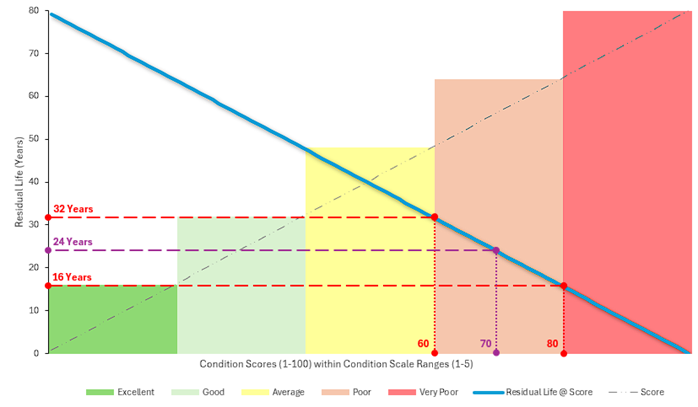
For example, consider the above raw Condition of 70, and Useful Life of 80 years. The raw Condition score intersects
the ‘Condition 4’ Condition Scale and thus has score range of 80 to 60. The lower/upper estimates are therefore:
Upper Age: 60% x 80 years = 48 years
Lower Age: 80% x 80 years = 64 years
Upper Residual Life Estimate: 80 years - 48 years = 32 years
Lower Residual Life Estimate: 80 years - 64 years = 16 years
The following graph shows how raw Condition Scores (1-100) within standard Condition Scales (1-5) interpolate
to provide a calculated Residual life with lower and upper range estimates. Figures from the above example have
been highlighted for clarity.
The above image shows the interpolation of calculated Residual Life values from raw Condition Scores and Condition
Scales.
Configuration
The Residual Life Report has support for the following configuration options:
Effective Date for Residual Life Calculations
The date to use for calculating the residual life values, relative to each component’s useful life.
When “Use Condition Record Date per Component” is selected, the effective date will be determined by each
component’s latest condition record date within the specified condition date limits.
Data filter
The predefined filter to use in restricting the data returned by the report.
Condition Selection Criteria
There are several Condition Selection Criteria that can be used to ‘refine’ the type and scope of Condition
Assessments you wish to require to satisfy this report. It is important to note that (unless explicitly requested)
the Condition Selection Criteria will NOT limit the Components that are exported by the report. Rather, it limits
what Condition records are considered valid for the report. The criteria include:
Condition Date Range Upper Limit
The latest condition record date to consider when selecting condition records for residual life calculations.
Condition records captured after this date will be excluded. Please note that this does not exclude
components from the export, rather, it simply limits what condition records are considered relevant when
calculating residual life. Clearing this value will default it to today.
Condition Date Range Lower Limit
The earliest condition record date to consider when selecting condition records for residual life calculations.
If left blank, all condition records prior to the upper limit will be considered. Please note that this does
not exclude components from the export, rather, it simply limits what condition records are considered
relevant when calculating residual life.
Condition Function Limitations
Select the condition function(s) as a filter for condition records to use for residual life calculations.
Only condition records captured against the selected function(s) will be considered. Please note that this does
not exclude components from the export, rather, it simply limits what condition records are considered relevant
when calculating residual life. No Exclusions when Blank.
Exclude Components without Condition Records
Components with no condition records matching the specified criteria will NOT be exported.
Enabling this will exclude any components that do not have condition records matching the specified criteria.
It should be noted that, even with default criteria, some components will not have a valid condition record
and will be excluded by this option.
Output
Depending on the report configuration options above, the Residual Life Report will generate the following
fields. Fields marked with an asterisk are compliant with reimportation for Component Updates.
Component Record ID *
The unique identifier for the Component record. This field is also vital for importing the dataset as a
Component Update.
Intervention Residual Life *
This is the calculated Residual Life of the Component, based on the most relevant Condition record, as
per any Condition Selection Criteria. The field name is consistent with the Component Update Import template
for modifying a Components Residual Life value.
Lower Range Residual Life
This is the calculated lower range Residual Life of the Component. This value is predicated on the ‘worst-case’
scenario of the relevant Condition Scale.
Upper Range Residual Life
This is the calculated upper range Residual Life of the Component. This value is predicated on the ‘best-case’
scenario of the relevant Condition Scale.
Intervention Useful Life *
This is the Component’s useful life value. It is included in the report to provide users with context for the
Residual Life calculations.
Effective Date *
This is the date in which the calculated Residual Life is ‘effective’ from. Report configuration options can
alter this value. When performing an update on Residual Life values, the effective date gives the context
of ‘when’ the change applies from; this is vital because Residual Life changes over time.
Effective Date Basis
This is an informational field detailing the way the effective date was set in the report’s initial configuration
options. It will be either ‘Condition’ or ‘Custom’. If ‘Condition’, it indicates that the date of the
Condition Assessment is being used (per-component) as the effective date of Residual Life calculations.
A ‘Custom’ basis indicates that the user supplied a fixed date for calculating Residual Life values.
Residual Life as at Effective Date
This value is included to provide the user with context around what the Component’s Residual Life value would
be at the supplied/derived effective date (above) without any data alterations.
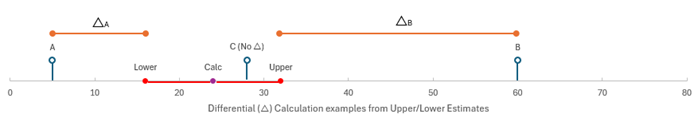
Residual Life Range Differential as at Effective Date
This value is included to provide the user with context around what the difference between ‘current’ values
and calculated values are. It is important to note that comparisons are always made to the upper/lower
bound estimates, rather than the calculated Residual Life. The graph below highlights the measurements
that this figure indicates.
In the above graph, the following is occurring:
Point ‘A’ falls below the lower estimate, therefore its differential is calculated from the lower estimate.
Point ‘B’ falls above the upper estimate, therefore its differential is calculated from the upper estimate.
Point ‘C’ falls within the lower/upper estimates, therefore there is zero differential.
Residual Life as at Now
This value is included to provide the user with context around what the Component’s Residual Life value
is as at the date of generating the report. This does not reflect the the supplied/derived effective date (above).
Selected Condition Record Function
This value indicates the underlying Condition Function used for the Component’s relevant Condition Assessment.
Essentially, it indicates the method of Condition Assessment per-row.
Selected Condition Record Date
This value indicates ‘when’ the relevant Condition Assessment was conducted. Note; if the ‘Effective Date Basis’
is set to ‘Condition’, this value will also be the ‘Effective Date’.
Selected Condition Raw Value
This is the underlying raw score for the relevant Condition Assessment. This is used to derive the Useful
Life multiplier for Residual Life calculations.
Selected Condition Value
This is the ‘scaled’ Condition value of the relevant Condition Assessment. Until the report supports custom
‘Condition Scale’ inputs (coming soon), it will always be a value between 1-5.
Condition Curve
This field is a placeholder for an upcoming feature that will permit users to define a custom relationship
between raw Condition scores and Life Multiplier values. Until the report supports such custom ‘curves’
(coming soon), it will always be ‘Straight Line’.
Condition Curve Life Multiplier
This field is a placeholder for the abovementioned ‘Condition Curve’ feature that will permit users to
define a custom relationship between raw Condition scores and Life Multiplier values. Until the report
supports such custom ‘curves’ (coming soon), this value will always reflect the ‘Straight Line’ calculation
metric described in the ‘Core Functionality’ section of this guide.
Selected Condition Functions
This is an informational field that reflects the reports underlying Configuration options. If the user
selects one or more ‘Condition Functions’ in as ‘Condition Function Limitations’, they will be listed
here. Otherwise, this field will state, ‘No Restrictions’.
Condition Scale Used
This is an informational field that reflects any constraints placed on the ‘Condition Scale’ used in
calculating the lower/upper estimates. This is a placeholder field and will always state, ‘System Default’
until custom Condition Scale selections are supported by the report (coming soon).
Warnings
This field may contain one or more messages per-row. These predefined messages are aimed at picking up
known scenarios that may be pertinent to the Component’s current state. The following are considered:
Missing construction/intervention date.
Construction/Intervention date greater than effective date.
Could not calculate residual life value as intervention useful life is missing.
Could not calculate residual life value as condition value is missing or no condition matches criteria’.
Residual life as at effective date is outside condition range residual life bounds.
Coming Soon
Due to the beta status of this report, there are a couple of features that have yet to be fully
rounded out, and as such, are flagged as ‘Coming Soon’. The following gives a brief overview of
these features.
Condition Curves (Ageing Profiles)
Condition curves will allow sites to define custom relationships between condition raw values (1-100)
and the corresponding life multiplier values. As detailed throughout this guide, the current methodology
for ageing profiles is ‘Straight Line’ where each increment in raw condition score, reflects a like
decrement in the life multiplier.
Condition Scales (Bounds for Estimations)
Custom condition scales, aside from enabling sites to define condition ranges such as 1-10 (or similar),
will also enable sites to have some control over the scale of upper/lower bounds for life estimates.
That is, if you control the range of raw condition scores covered by a condition’s corresponding scale,
then you also control the upper/lower estimates for residual life.
How To Guides
This section provides an overview on the following Report Generation topics:
To generate a new report in the Metrix Asset Management system, follow these steps:
Navigate to the ‘Reports’ page of the application.
Reports are grouped into sections of common themes and each report is represented by a tile with a label
and brief description. Click on your desired report. See Report Generation: About
for further information about specific reports.
The report configuration/preview page will load. Depending on the selected report template, a number of configuration
options may be present on the left, whilst on the right-hand side, a preview of the report will be shown. Make sure you
provide a setting for any required report configuration settings by scrolling through the left-hand side section.
Tip
Some reports will display additional options when certain configuration settings are switched. Try applying a ‘Custom Filter’
to the ‘Component Data Export’. The option to include ‘Custom Attributes’ will then be shown.
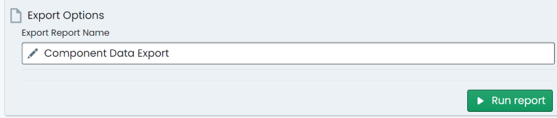
Once configured, update the name for your report (optional - a default name is pre-populated), and click ‘Run report’.
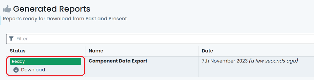
The report has now been queued for generation. The application will navigate to the generated reports page where past
reports are listed for download. At the top of this list, the report you just created will be listed with a status flag in the
left-most column. Once it is displayed as ‘Ready’, click the ‘Download’ option for that report.
Depending on your browser settings, you may be prompted for a ‘save’ location for the generated report. Save the file
to your computer. You have now generated and downloaded a report from Metrix.
Downloading Past Reports
Each report generated in the Metrix Asset Management system is available for download at any time, via the
‘Generated Reports’ page. To view and download a past report, follow these steps:
Navigate to the ‘Reports’ page of the application.
Click on the ‘Generated Reports’ option on the left-hand side of the page.
On this page, past reports are listed for download in a chronological order (by the date they were created). For
the report you wish to view, click the ‘Download’ option for that report.
Depending on your browser settings, you may be prompted for a ‘save’ location for the generated report. Save the file
to your computer.
Defining Report Factor Sets
The Metrix Asset Management system offers the
Cost to Bring to Satisfactory Report
as a built-in report template for users. This report calculates intervention metrics for components based on their
condition a pre-defined factor set. This guide details how to create and manage such factor sets.
Navigate to the ‘Reports’ page of the application.
From the report template list, select ‘Cost to Bring to Satisfactory Report’.
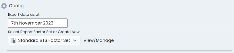
This will take you to the generation/configuration page for this report option. The current chosen ‘Factor Set’ will
be active in the ‘Report Factor Set’ drop-down. If you have never created your own ‘Factor Set’, this will be a system
default set.
To create a new ‘Factor Set’, select ‘Create New Factor Set’ from the drop-down list options. To edit the active ‘Factor Set’,
click on ‘View/Manage’ next to the drop-down list.
If creating a new ‘Factor Set’, enter a ‘Factor Set Name’ in the text input box. Then select the ‘Report Category’ for which
this ‘Factor Set’ will apply to. If editing, the existing ‘Factor Set’, click ‘Edit’.
For each option configured for the report category, an array of factors will be generate per scaled condition score of 1-5. These
are placeholders for you to replace with your actual factors. To set the factors, there are two options:
Set Globally
The top row of the list is reserved for global assignment. That is, this row does not pertain to a particular report category
option - it is there to allow you to set a figure that will be replicated across ALL report category options below.
Set Individually
Excepting the top row, each row represents a configured report category option. These rows can be individually managed by
inputting values directly.
First, choose a factor base as ‘Replacement Value’ or ‘Carrying Value’. This is the metric that will be multiplied by the report
factor per scaled condition score.
or each scaled condition score across the row, input the desired report factor from 0% to 100%.
When you have finished, click ‘Save’ at the top of the table.